An extension of the Walsh-Hadamard transform to calculate and model epistasis in genetic landscapes of arbitrary shape and complexity | PLOS Computational Biology

Andre J. Faure, Ben Lehner, Verónica Miró Pina, Claudia Serrano Colome, Donate Weghorn

PLOS CompBio 2024

5 Min overview of the setup –> key idea

Want to learn a sequence to scalar function map. Could just have a lookup table, but we want interpretability. Introduce all-orders model¹ as fitting any possible function on sequences (has coefficients on all possible terms), and being interpretable. What are these coefficients? Epistatic coefficients! We start from a definition of epistasis, write for L=1, s=2 which is intuitive to us in that it measures deviation from the null hypothesis of linear additivity of single mutations. However, this can (somewhat unintuitively) be rewritten as periodic mutational differences, reorganize terms to make this clear, M0 inside parens, M1 across parens, which turns out to be equivalent to the WHT which is just doing discrete spectral analysis. From here we can write background-averaged epistasis as the WHT with small scaling modifications, and the other two types as matmuls on top of that. The key innovation of the current paper then is to extend this from the binary case to multiple states per position. This is done by relatively simply extending the \(H\) matrix definition; we basically frame multiple states as multiple separate binary mutations from WT. For a fixed position, these are calculated separately of one another (like doing separate binary WHT), and for background-averaging over other positions, you get to average over multiple states, which is desirable. This is easily extensible to different numbers of states at different positions b/c each recursion corresponds to a single position, so the matrix can be expanded \(s\) times at a given recursion, where \(s\) is flexible. Computationally, they use linear regression to compute background-averaged epistasis (Walsh-Hadamard Transform does this for WT-reference instead), and provide formulas for extracting individual elements of any of the matrices, so you can compute specific terms or partial data regime or batch these computations for modern GPU parallelization. Main limitations are that it’s still super intractable to compute for higher-order terms, for longer sequences, for larger state spaces due to combinatorial explosion of terms. However, this is in some ways unavoidable if you want to estimate all coefficients, unless you knew sparsity structure a priori and could simply operate on fewer coefficients. Also limited in that usually in limited data regime for empirical landscapes, though WHT-on-predictions-(complete-landscapes) may also be a good use case for this. In this sort of regime, another alternative (or complementary method?) is aggregating epistatic orders, as one might do with the ANOVA kernel / Newton identities, to make more tractable.

5 Min overview REVISED

Want to learn a sequence to scalar function map. Could just have a lookup table, but we want interpretability. Introduce all-orders model¹ as fitting any possible function on sequences (has coefficients on all possible terms), and being interpretable. What are these coefficients? Epistatic coefficients! In a nutshell, we can write out intuitive formulas for epistatic coefficients that measure how much interaction occurs for a certain set of position-AAs. It turns out that for binary sequences (2 states) these formulas correspond to a slight modification of the WHT. Write relation \(\epsilon\) \(H\) \(y\) (w/ scaling mat) Write H recursive form.

The key contribution of this paper is to generalize the WHT to arbitrary sized state spaces per position. write new H recursive form This is basically framing (for a specific position) multiple states as multiple separate binary mutations from WT and computing ‘separate’ binary WHT for each, but then when we recurse to another position, we can background average over all states at the other position.

They also show that there’s an easy recursive form for the inverse of \(H\), which avoids having to construct \(H\) and then invert it (cubic time). This is relevant since often we expect to use WHT by LR. They also show that we can extract specific elements of \(H\), \(A\), \(V\) in the event that we want to compute only certain \(\epsilon\) or have missing data \(y\).

Experiments show that 1) their formulas yield computational speedups and 2) that they can extract ground truth epistatic coefficients pretty reliably at different (still large) data volumes.

Still limited in that intractable to compute for higher-order terms, for longer sequences, for larger state spaces due to combinatorial explosion of terms. Sorta unavoidable though and nice to have a concrete formalism for multiple states.

TODO

read about gauges: Gauge fixing for sequence-function relationships | bioRxiv Gauges

scan ref 28, 29

Newton-identities-/-ANOVA-application-to-WHT

Kernelizing? — still want to think more about, but maybe should wait until after exam. when can you kernelize? when you only want an inner product, instead of the actual embedding. when do i only want inner products of epistatic terms instead of the actual terms? is there a way i could kernelize so that I can extract nonzero epistatic terms only? or apply them in a way such that it’s evident? like taking the norm over various different embedding subsets to find nonzero elements. or does this increase computation back to the original problem, or more…

think about Alternative-idea-(mine)-compare-to-avg-of-other-AAs-@-position-instead-of-WT some more — I think what I’m proposing is effectively using zero-sum gauge instead of WT gauge. Are there easy ways to transform between WTG and ZSG? See also Insight-from-Gauges.

think about statement: full background unlikely to be useful for enhancing in neighborhood of WT bc much of landscape likely dead (though this should strengthen good signal, right? but may be harder to distinguish between WT and stuff better than WT if WT > avg). I think reading about gauges is helping with this —> Gauges

think about opt approach w/ min L1 norm \(\epsilon\) s.t. \(y=H^{-1}V^{-1}\epsilon\) — how do you do this practically? a la cvxopt? (maybe from Walsh-Hadamard Transform paper) —> Walsh-Hadamard Transform#Sparse optimization approach

Optimization,-FGMs

Plausible questions

• Explain equations 24, 25
• Explain Fig. 1
• Explain Fig. 2
• Write down the binary WHT setup
• How does the WHT connect to epistasis?
• How is the WHT changed to accommodate epistasis interpretation?
• How is the WHT generalized to multiple states per position?
• Write down the gWHT form.
• How is epistasis defined? Write an example equation for a simple \(L=2, s=2\) example.
• How would you do binary genotype —> phenotype mapping without the WHT?
• How would you do multi-state genotype —> phenotype mapping without the gWHT?
  • Naive dimension is \(D^L\)
  • OHE, make each possible state for each position binary meaning \(2^{D\cdot L}\), this is impractically large and is an inefficient representation.
  • Graph fourier basis, basically for each position get vector of size \((d-1)^L\) but lose interpretability, mathematically complex
• Can you explain Table 1?
• What is the form of the inverse matrix?
• Prove that the recursive inverse matrix form is actually the inverse of \(H\).
• Why do we care about extracting single entries?
• What do we do if we have missing data?
• What do we do if we only want to model a subset of epistatic coefficients?
• Write the formula for getting a single element of \(H\). Of A? Of V?
• How can I generalize this to have different numbers of states at each position?
  • How does this change \(H\), \(A\)?
• How do they get the epistatic coefficients in their experiments?
• What is one-hot-encoded model baseline?
• What are existing limitations of this approach?
• Motivate this approach.
• How might you improve this approach?
• How might you extend this approach?
• Why can’t we do WHT in terms of the ZSG / without a reference sequence?
• Write the LR formulation for WHT

From Perplexity

Conceptual Questions

1. What is the significance of extending the Walsh-Hadamard transform to multiallelic landscapes?
2. How does background-averaged epistasis differ from other forms of epistasis, and why might it be particularly useful?
3. What are the limitations of the original Walsh-Hadamard transform in the context of genetic landscapes?
4. How does deep mutational scanning (DMS) contribute to the study of epistasis?
5. Why is it important to model epistasis in genetic landscapes?
6. How does the concept of “background-averaged” epistasis relate to Fisher’s “statistical epistasis”?
7. What are the potential applications of this extended Walsh-Hadamard transform in fields such as protein engineering or evolutionary biology?
8. How does the approach presented in this paper differ from alternative implementations for multiallelic landscapes?
9. What is the significance of being able to extract epistatic coefficients without constructing or inverting large matrices?
10. How might this new method impact our understanding of the relationship between genotype and phenotype?

Technical Questions

1. Explain the mathematical representation of a genotype sequence used in this paper.
2. How is the phenotypic effect of a genotype typically measured in empirical genotype-phenotype landscapes?
3. Describe the calculation of a pairwise epistatic coefficient in a background-averaged context.
4. What is the role of the ^V matrix in the Walsh-Hadamard transform?
5. How is the ^H matrix (Walsh-Hadamard transform) defined recursively?
6. Explain the mathematical formulation for extending the Walsh-Hadamard transform to sequences with an arbitrary number of states s.
7. How does the paper define the simplest possible multi-state (multiallelic) landscape?
8. What is the significance of the formula εn = ^Vn · ^Hn · yn?
9. How does the paper propose to extract elements of the transform matrices without constructing or inverting large matrices?
10. Describe the mathematical approach used to derive the inverse matrix for inferring epistatic coefficients using regression.

From chatGPT

Conceptual Questions

1. What is the main motivation for extending the Walsh-Hadamard transform to multiallelic genetic landscapes?
2. How does background-averaged epistasis differ from statistical epistasis as defined by Fisher?
3. Why is the study of epistasis important for understanding genotype-phenotype mappings in biology?
4. What are the limitations of the traditional Walsh-Hadamard transform when applied to genetic landscapes?
5. How does this new extension address the challenge of modeling multiallelic landscapes with missing data?
6. Why are pairwise and higher-order genetic interactions relevant for phenotypic prediction?
7. What role does deep mutational scanning (DMS) data play in this study of epistasis?
8. How does background-averaged epistasis enhance our understanding of direct physical interactions in biomolecules?
9. What are the potential implications of this research for synthetic biology and protein engineering?
10. In what ways might this extension of the Walsh-Hadamard transform influence future research in evolutionary biology?

Technical Questions

1. Can you explain the recursive formula provided for the inverse matrix and its significance?
2. How does the paper handle the computational challenges associated with large-scale genetic landscapes?
3. What is the mathematical rationale for introducing zero elements in the multiallelic extension of the Walsh-Hadamard transform?
4. Describe how sparse regression models are used to infer background-averaged epistatic coefficients.
5. What is the significance of the normalization matrix VVV in the Walsh-Hadamard transform framework?
6. How do the authors demonstrate the utility of their theory using simulated and empirical datasets?
7. What are the key benchmarking results for the computational performance of the proposed methods?
8. How are elements of the matrices HnH_nHn​ and AnA_nAn​ obtained directly, and why is this feature important?
9. Explain how Lasso regression is applied to model background-averaged epistasis in the context of missing data.
10. What evidence does the paper provide to show that background-averaged models generalize well, even with sparse data?

Basic WH formulation? (p 1-4)

From Poelwijk et al. paper

Alternative approaches to gWHT (p 3)

Alternative representation

Alternatives to present work for generalizing to multiple states: one-hot encoding², graph Fourier bases³. My naive understanding is that once converted to these bases, a standard binary WHT can be easily run. However, may face dimensionality blowup.

Alternative higher-order interaction modeling

Only scanning these references. From same first/last authors, 29 is from 2020 and 28 is from 2022.

Ref. 29: Minimum epistasis interpolation for sequence-function relationships

Goal

Impute function values for genotypes not measured.

Approach: min. epistasis interpolation

Infer the least epistatic possible sequence-function relationship compatible with the data. This ends up being equivalent to additive (nonepistatic) modeling?

Details

Want mutational effects to change as little as possible between adjacent genetic backgrounds. To avoid dealing with sign of \(\epsilon\) (depends on which sequence is chosen as WT), they use \(\epsilon^2\) instead. Then, choose prediction \(\hat{f}\) that minimizes \(\epsilon^2\). In the 2-position binary case, this means the prediction for double mutant would be sum of single mutations. In general, they consider the hypercube that is the Hamming graph and look at each “face” consisting of a “WT”depends on which sequence is chosen as WT two single mutants, and a double mutant. This is fully general in the sense that the WT changes on each face. From each face can get an \(\epsilon_i^2\) and can minimize sum/average over all faces⁴. B/c all non-negative and formula for \(\epsilon^2\) is polynomial, actually have an SDP with an equality constraint⁵ that has an analytic solution. Number of linear equations to solve scales cubically w/ # of unobserved genotypes, so can apply if less than a million but for longer sequences, cannot. For example, \(20^5\) is probably already too much @ 3.2M. Can actually kernelize the problem to remove exponential dependence —> linear in \(L\) and cubically in \(n\) number of observations; they report up to 20,000 observed sequence limit.

Properties

For any missing genotype, prediction is equal to average local “nonepistatic”⁶ prediction (over other three genotypes in faces it shares)⁷. Can interpret as a Taylor approximation around missing genotype, where we estimate with mean value of Hamming distance 1 sequences, and correct this with the difference btwn this mean value and the mean value for Hamming distance 2 sequences. Intuitively, this is the network effect of being in multiple faces all of which neighbors are in other faces too. Fig. 4 seems informative.

Ref. 28: Higher-order epistasis and phenotypic prediction

Goal

Impute function values for genotypes not measured. Use epistasis as an intermediary to ground these predictions. Principles: 1) Try to use all orders of interaction 2) Observations in nearby genetic backgrounds should influence predictions more than those far away (this will come from the prior, I expect)

Approach: higher-order epistasis prior matching

Make predictions for unobserved genotypes that match the type and extent of epistasis found in the observed data. To get this info, will consider how function value correlations change as a function of mutational distance, or equivalently, estimate fraction of variance coming from each order of genetic interaction. With this, we can fit an empirical Bayes prior that matches observed epistasis, do GPR under this prior.

Details

Fig. 1 is interesting — shows that the correlation as function of Hamming distance falls off more quickly for higher-order interaction terms, which makes sense intuitively. Note that this is in aggregate, and I’m not sure what you’d expect if there’s e.g., one really strong higher-order interaction term that permeates the landscape substantially. But I guess if you expect ruggedness, this shouldn’t matter too much. Should read more on Krawtchouk polynomials in this context, seems like an interesting (but complex) idea. Have to use HMC to draw samples from GP posterior (why?) and can make predictions for up to low millions of sequences. Not sure what constraint on training data is, but expect it to scale cubically too b/c GP. Seems interesting, would need to read the SI to know more.

Multiallelic WHT (p 5-8)

Example \(n=1, \;s=3\): \(\epsilon_{*} = \frac{1}{3}\cdot (y_{0}+y_1+y_2),\; \epsilon_{1}= (-1) \cdot (y_{0}-y_{1}),\; \epsilon_{2}= (-1) \cdot (y_{0}-y_2)\) This is a somewhat trivial generalization of the WHT where we just compare our different mutations at the same position to WT separately.

\(n=2\), \(s=3\): 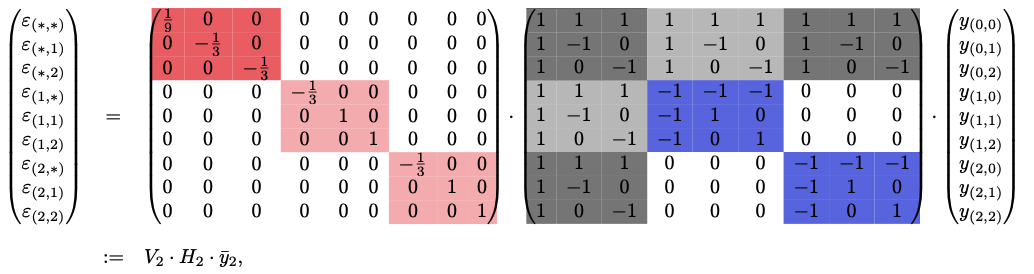^5a2740

Alternative idea (mine): compare to avg of other AAs @ position instead of WT

is comparing each mutation to all other AAs @ that position, instead of just WT. Concretely, this would look like: \(\epsilon_{1}= (-1) \cdot (\frac{y_{0}+y_2}{2}-y_{1}),\;\epsilon_{2}= (-1) \cdot (\frac{y_{0}+y_1}{2}-y_2)\) or potentially, the average could include all function values. Not quite sure what this looks like in extension to recursion depth \(\gt 1\). Let’s consider an example. For reference, from binary Walsh-Hadamard Transform: \(\epsilon_{1,1} = (y_{1,1} - y_{0,1}) - (y_{1,0} - y_{0,0})\). \(\epsilon_{1,1}= (-1) \cdot ((\text{avg}(y_{0,1},y_{2,1})-y_{1,1})-(\text{avg}((\text{avg}(y_{0,0}, y_{2,0}) - y_{1,0}),((\text{avg}(y_{0,2}, y_{2,2}) - y_{1,2}))\) (I’m not fully sure if this is correct, and am generally confused). Easier to think about wrt colored matrix figure in the paper. Here, we find effect of a mutation in P0 (avg over mutating from WT 0 and other AAs) in context of all AAs @ other positions. Then find effect of next mutation in P1 by subtracting off average of effects of mutation0 over other AAs @ P1. This is doable, but maybe not trivially in current WHT setup. May have to tinker with scaling matrix to do multiple averages. However, may be amenable to FWHT-type algo. Unsure.

Notice that for the “reference”, we allow mutations from any other AA @ relevant position while holding the other position fixed, since we’re interested in knowing how this mutation behaves in the context of another mutation. What if we have different AA identities at the positions being considered?

It’s not really clear to me why this shouldn’t be done. Potential reasons: 1) This will average out signal too much. A mutation may be positive vs. WT, but have no signal vs. average. Maybe a matter of priorities – do we want to do better than a reference, or better than average? Do we have data to power us to do better than WT, or average over all positions? 2) Computationally / algorithmically more complex. And, may be equivalent under some gauge change (unsure, need to read about this). 3) I really am interested in finding a difference relative to a WT, b/c I want a clear (singular) explanation. Mutational interactions vs. WT has clear interpretation, but mutational interactions vs. average just tells you that these interactions are important, though they may be present in parts in the reference (average).

Insight from Gauges

It turns out that you’re not limited to a strict WT gauge (which is what WHT does by default), and while you could try to average over all positions, which in the limit would get you the ZSG, you can also define a generalized WT gauge by specifying a distribution on multiple AAs @ a certain position (with some still allocated 0 prob. mass). This is computationally easier in this setting — this would be akin to selecting multiple relevant baseline sequences / WT, and then averaging over all of those, instead of all possible sequences. Specifically, you’d only average⁸ certain terms at certain recursion levels / positions. And then interpretation of this may make more sense b/c you’re tethered to the WT set you chose.

Is this equivalent to doing a bunch of separate binary WHT?

My current intuition is that this ignores other AAs at the position being considered, but will background-average over all AAs @ other positions, which is desirable. Meaning on a per-position basis, it’s still the same old binary WHT. But we compute this binary WHT for all AAs @ that position. And then we background average over all AAs @ other positions. See Generalized Walsh-Hadamard Transform#^5a2740 for example matmul. Background averaging only occurs when there’s a \(*\) in epistasis term and it happens precisely over all values that \(*\) could take on. This is why we see for the first 3 terms, inclusion of all* \(y\) values.

gWHT scaling matrix and full matrix formulation (p 7)

Scaling matrix \(V\) looks analogous to the one in Walsh-Hadamard Transform combined with the sparsity structure of \(H\) defined here, with the only difference being now the first row is scaled by \(\frac{1}{s}\) b/c we want an average (before was \(\frac{1}{2}\) b/c only 2 states).

Putting this together, we write background-averaged epistasis (again) as \(\epsilon=(V\cdot H)\cdot y\). This requires having all \(y\) values!

Linear regression view, revisited (p 7-8)

If don’t have \(y\) for all genotypes up to desired order, can take linear regression view again. Here we say that \(y = H^{-1}\cdot V^{-1} \cdot \epsilon\). We can precompute the matrix inverses, and then compute \(\epsilon\) given \(y\). The paper says that this is “analogous” to the OHE strategy (which implicitly uses background-relative view when regressing) – not sure what this means. As far as I can tell, when regressing, there’s no reason in particular you have to be background-relative. But now, actually, I remember that this was a transformation on top of background-relative in Walsh-Hadamard Transform. Ok, in that paper, this is true; however, it’s not clear that the linear regression view must be based upon background-relative and one could imagine removing that matrix to have a background-averaged LR setup. There’s a second question of whether you’d be powered to do that, and perhaps zeroing out everything other than WT-relevant terms is an easy way to do this. Recall that b/c LR, we want \(n\) number of datapoints > \(r\) number of coefficients, or there will be infinitely many solutions. This paper has simply defined LR in this manner, unclear if there’s any fundamental reason cannot do other way by shifting \(X\) so it’s not equal to \(G^{-1}\). No; actually, equivalence to \(G^-1\) falls out of the definition of \(X\) which is based on the LR formula. \(X\) simply selects with coefficients should be added up to compute each \(y\), which doesn’t have consideration of WT vs. BA in any way that’s clear to me, meaning that formulating in this manner is just implicitly equivalent to WT for reasons beyond me. Confusion again– Equation 13 is actually introducing the inverse matrices required for LR w/ background-averaging, as it just uses \(H\) instead of zeroing out any WT stuff, such that all epistatic terms are used in the computation of all \(y\) values. This seems more confusing to interpret, though. ==Gauge-choice relevance again?==

Extension to different numbers of states at each position (p 10)

It’s easy to extend to different numbers of states at each position. Define \(s_i\) as the number of states at position \(i\). Then each recursion layer simply applies the previous matrix that number of times. \(H_1\) will be \(s_{1} \times s_1\). \(H_2\) will require \(s_{2}\times s_2\) blocks of \(H_1\). Overall, the size of matrix for length \(L\) will be \(\prod_{i=1}^{L} s_i \times \prod_{i=1}^{L} s_i\). Can do Obtaining-individual-elements-of-matrices-(p-8-9,-10) in effectively the same manner as normal.

Computation (p 8-9)

Obtaining individual elements of matrices (p 8-9, 10)

^641807 This is generally desirable if you only want certain elements, for LR case, and also for batching on modern GPU, which may incur speedups that outweigh any losses from extra computation done here.

Meta-remarks

I don’t understand their indexing scheme or why it needs to be introduced at all. Upon reflection, I suspect it’s basically saying to index the matrix the same way the \(y\) vector is indexed, on both row and column axes. This way we can interpret entries in the matrix as corresponding to certain genotype combinations, though I’m not sure why we want to do this / this isn’t inherent to \(H\) or any of the matrices (they’re just, square⁹).

Note also that this should extend straightforwardly to the binary WHT.

Formulation

Want to write \((H_n)_{ij}\). Define \((E_n)_{ij}\) to be the number of positions at which sequences \(i\) and \(j\) carry the same mutated allele. Define \((M_n)_{ij}\) as the total number of positions where sequences share the same allele, meaning \((E_n)_{ij}\) plus shared WT positions. Then we can write \((H_n)_{ij} = 0\) if \((M_n)_{ij} \neq n\); \((H_n)_{ij} = (-1)^{(E_n)_{ij}}\) if \((M_n)_{ij} = n\). We can similarly write the inverse of \(H\), \(A\), in terms of only \(E\). We can write \(V\) and \(V^{-1}\) in terms of \((W_n)_i\) (note only \(i\), not \(ij\), b/c \(V\) matrices are scaling and only have diagonal elements, i.e., \(\{i,i\}\)), which is the number of positions in \(i\) carrying WT allele. Note WT-relative is baked into all of the above.

Interpretation

We can get single elements of \(H, A, V, V^{-1}\), which allows us to compute single epistatic terms by e.g., finding the appropriate scaling term and computing the relevant row of \(H\). In the LR case, this may also allow you to more easily specify present vs. dropped rows based on which genotypes you have \(y\) for (?). Overall, these just fall out of the recursive definitions of \(V, H\). Can be proved by induction and are in the SI, but don’t think the proofs are very instructive to me.

Indexing: basically the order of \(y\) (according to \(x\)), then map that over the row and column axes of the matrix.

For \(H\): 0 if there’s an index where at this position, the indices give different mutations — basically saying that we never want to compute within-position mutation differences b/c we’re interested in doing multiple binary WHTs. Otherwise, the sum of WT positions on either combined w/ shared mutations will equal \(n\), and negative / positive 1 is decided by how many shared mutations. If none shared (like first row/column) then 1. If 1 shared (like diagonal) then -1. If 2 shared (recursive depth=1) then get flipped back to 1.

For \(A\): each time a specific mutation is shared, you end up on the diagonal of \(A\), so you multiply by \((1-s)\). This formula just exponentiates by the number of times that happens.

For \(V\): always a diagonal matrix. Diagonal elements are just \(\frac{1}{s}\) exponentiated to how many times WT is present, and negativity based on how many mutations are shared (which is just \(n-W\) b/c we’re on the diagonal).

Benchmarking performance

Fig 1E, F demonstrate that for both compute time and memory usage, recursive building \(H\) and \(A\) is better than doing all elements (in the style ofObtaining-individual-elements-of-matrices-(p-8-9,-10)), but that you can extract a constant number of matrix elements for an effectively constant price. The per-element price is higher, unsurprisingly, due to needing to compute \(E\)¹⁰, which is reflected in “all elements \(A_n\)”. Moreover, by recursively constructing \(A\), you can get speedup over recursively building \(H\) and then inverting it, which isn’t surprising, but is meaningful for Linear-regression-view,-revisited-(p-7-8), which appears to be what most cases call for in practice.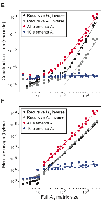 Cites full construction of \(A_4\) for protein (\(s=20\)) would take \(\gt 10^{20}\) bytes memory; however, using only up to third-order terms and extracting the subset of elements¹¹ needed for prediction¹² of a single phenotype can be done w/ 192 GB memory in 99 seconds. Seems somewhat tractable.

Experiments (p 11-15, 16-18)

Experiment setup

Have some multiallelic landscape. Experiments will measure three main things: 1) % variance explained (on test data) by learned epistatic coefficients, varying with amount of training data used (from 1% - 64%). Compared to onehot binary WHT approach. This is computed in some strange way using their earlier work called DiMSum. However, I think this could be computed using \(R^2\) to same effect¹³. 2) Correlation to ground-truth epistatic coefficients (if available) or reported (experimental?) values. 3) Enrichment of direct physical interactions in nonzero epistatic coefficients predicted. An odds ratio is used between binary indicators for both variables. Let \(N\) be the probability that a position pair (of all possible) has nonzero epistatic coefficient. Let \(D\) be the probability that a position pair has direct physical contact. Interpretation is “odds of D occurring in presence of N over odds of D occurring in absence of N” (really, both ways would make some sense)¹⁴. Then \(OR = \frac{D\cdot(1-N)}{N\cdot(1-D)}\). Compared to onehot binary WHT approach.

All models trained here are Lasso linear regression onto the epistatic coefficients. 10-fold CV is performed to select \(\lambda \in [0.005, 0.25]\).

Simulated landscape

\(L=6\), \(n=4\) so total \(4^6=4098\) genotypes. Draw first order, and some second order epistatic coefficients from Gaussians¹⁵. Others are set to zero¹⁶.We can then use these ground truth coefficients for evaluation. Simulated fitness values can be easily constructed using \(y = H^{-1}\cdot V^{-1} \cdot \epsilon\). Noise is added of similar scale to first-order coefficients, lower and higher noise in SI B. They perform Lasso linear regression with coefficients up to 3rd order.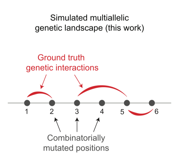

Experimental landscapes

Two empirical combinatorial fitness landscapes. For tRNA, \(L=10\) and \(s=\{2,3\}\). They only regress up to 8th order coefficients. For eqFP611, \(L=13\) and \(s=2\) and they regress up to 3rd¹⁷ order coefficients¹⁸. Note that “ground-truth” epistatic coefficients in these cases are just previously reported background-averaged epistatic coefficients, which were computed using some binary WHT extension or other. 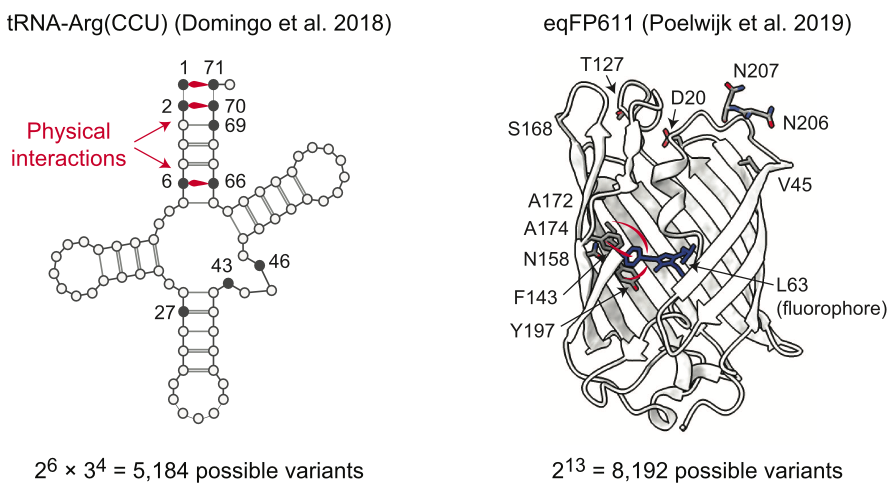Interestingly, they actually impute values for missing data so that they can do the normal full gWHT. Similar to Hunter idea / discussion @ FGM GM. This direction is making me wonder if using this (or FGM) on model predictions / large model auditing would make sense.

Results

1) We notice that at best (64%), we get about 60-80% of variance explained. However, the drop off isn’t terrible, even at 1% or other single digits. Still, for larger landscapes of the sort we’d generally like to examine, tractability is not the rule¹⁹. 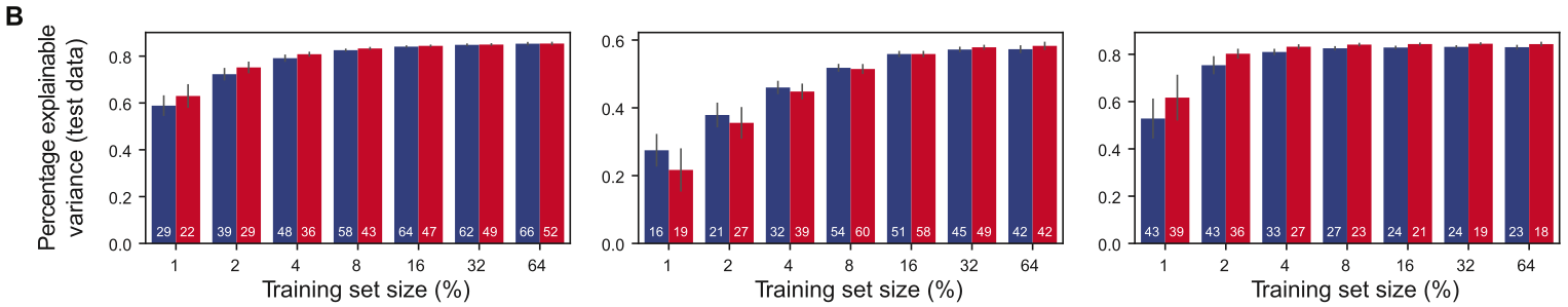2) Pretty small number of nonzero coefficients overall, though. These plots only show coefficients up to 2nd, 3rd order²⁰. 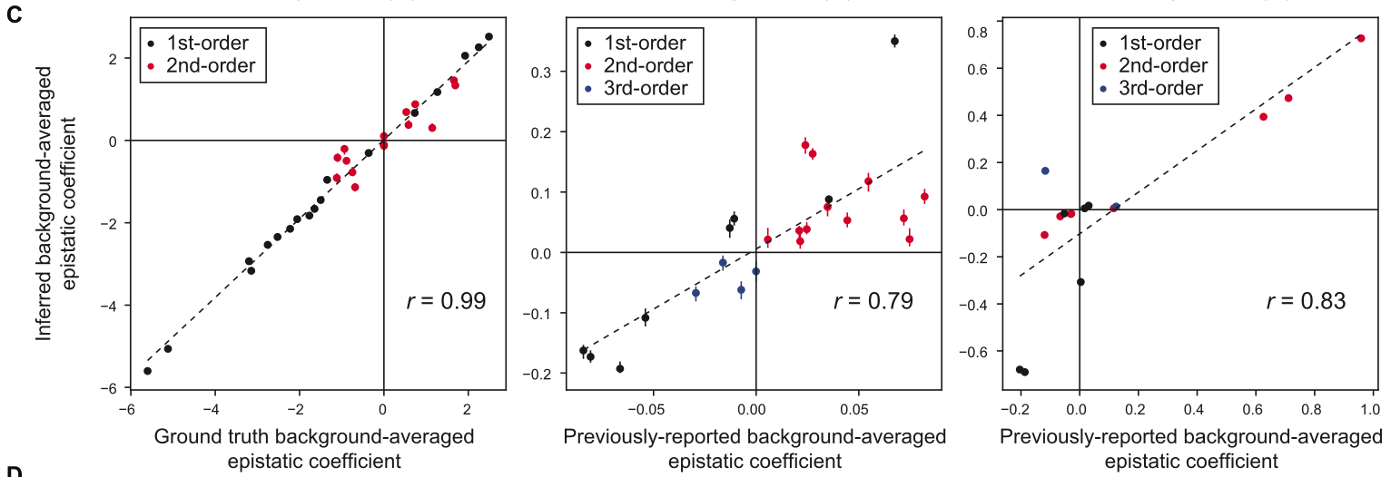3) Here, we compare enrichment for nonzero epistatic coefficients corresponding to residues in direct physical contact. Note that background-averaging does better than OHE across training set sizes, though the trends aren’t totally clear²¹.

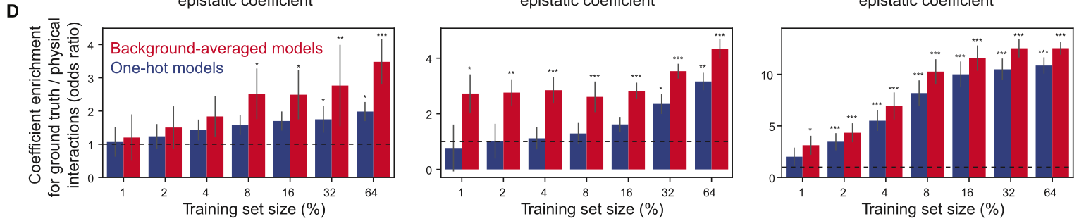
Discussion (p 15-16)

The new gWHT provides a matrix \(H\) that is not necessary orthogonal (as is the case for the binary WHT). The columns of \(H\) are still independent (i.e., can still compute inverse, \(A\)).

Connections

Gauges

Want to read about gauges and think about epistasis as WT-gauge²². This is relevant because in the generalization mutation is always defined w.r.t. WT, even if it’s averaged over arbitrary backgrounds. This means that there isn’t really any interaction between different mutations at the same position in this computation.

Q: Is full background unlikely to be useful for enhancing function in the neighborhood of WT b/c much of the landscape away from WT is likely dead? → This should strengthen good signal instead, right? → May be harder to distinguish between WT and stuff better than WT though, if WT > avg. → This is actually the tradeoff in interpretability between the WTG and the ZSG. The WTG gives everything relative to WT, so things better than WT (of which there may be very few) should show clear signal. Otoh, the WT may be massively positive relative to the average in the ZSG, meaning sequences better than WT may not be super distinguishable from the WT. What we really care about here though is how interpretable the parameters under these different gauges are. If your goal is to do better than WT, my intuition is that WTG is still better, as params are all defined as effects of mutating WT (instead of effects of mutating from “average”).

Newton identities / ANOVA application to WHT

Q: why can’t we apply newton identities (or ANOVA more generally) here to aggregate epistatic orders? does this just not fit into any WH formalism? Is the gain really from kernelizing, like Renzo / Jenn seemed to think? Ref.-28-[Higher-order-epistasis-and-phenotypic-prediction](https-//www.pnas.org/doi/full/10.1073/pnas.2204233119) mentioned kernelizing. → In trying to have an epistatic model, we need to be able to fit / compute a coefficient for every term in the full all-orders interaction model. Using ANOVA or something of the sort would not allow fitting of these coefficients; you could only compute or fit coefficients on the order level. Aggregation pre-coefficient fitting/computation isn’t really helpful because then your model isn’t powerful enough.

Kernelizing?

Is the gain really from kernelizing, like Renzo / Jenn seemed to think? Ref.-28-[Higher-order-epistasis-and-phenotypic-prediction](https-//www.pnas.org/doi/full/10.1073/pnas) mentioned kernelizing. How would we kernelize the WHT? What does this question even mean?

Optimization, FGMs

Given (sparse, or sparsified) epistatic coefficients up to arbitrary order, can now construct an “interaction graph” analogous to an FGM: edge absent only if \(i,j\) are not together in any nonzero interaction term. This actually helps to highlight how FGMs and epistasis computation are different: epistasis is much, much more information. If I try to define a criteria for adding an edge: naively, if \(i,j\) are together in any nonzero interaction term. But this clearly throws away a ton of information I have about what those interaction terms are. For example, imagine a third order term that’s encapsulated by a fifth order term. FGM thinking would say that you have to optimize all five together. Epistasis might tell you that you should consider all five together, but that moreover, three of the five interact in some way that contributes to function differently than five. In FGM land, you would hope that your regressor on all five would figure this out, but it seems likely better to have a regressor on the three terms and a regressor on the five terms separately, that get added up, for parsimony’s sake — this way the three term regressor can account for that interaction, and the five term regressor need not, and can focus only on the fifth order interaction effect. Overall, I think this could still use more thought.

WHT on predictions (complete landscapes)

Can we use something like WHT on a complete landscape for interpretability or for regularization of the network?

Misc

Footnotes

1. Still has same number of terms as lookup table, but here multiple terms contribute to each of the function values, so we have some sense of generality. ↩ ↩²

2. On the sparsity of fitness functions and implications for learning | PNAS – OHE makes categorical data binary, can then naively apply WHT to. Even this isn’t totally clear to me though – WHT requires all possible binary strings up to an order, meaning you could only use the linear regression approach on OHE data, unless you modify the structure of \(H\) to zero out indices corresponding to other AA options at a certain position. This will be very inefficient though because the size of the space goes from \(20^L\) to \(2^{20^L}\) (on or off for each position, for each AA option) which is obviously much larger. This difference in efficiency comes from the fact that only one of the 20 indices corresponding to a given position can be on (1) at a time. Note, importantly, that this implicitly uses a background (WT)-relative view because each index is binary w.r.t. the WT?? ↩

3. Skip reading about for now, but discussed in On the sparsity of fitness functions and implications for learning | PNAS as well, and in more detail. ↩

4. Though, how many faces will there be total for a reasonably sized landscape? Does this encounter tractability issue? In some sense, they’ve reduced the whole landscape to pairwise terms, similar to FGM-type approach. ↩

5. To existing datapoints. ↩

6. additive model ↩

7. Unclear if this is meant for all faces it’s a part of, though seems to suggest. That is indeed surprising and unintuitive to me, then. ↩

8. This would not be a straight up (uniform) average, I believe, but rather an expectation relative to the chosen probability distribution (b/c finite state space, a probability mass-weighted sum where some terms are zeroed out). ↩

9. sans generalization to different numbers of states at each position… ↩

10. This seems easily pre-computable for a variety of sizes of \(H\) matrix. ↩

11. Assuming that both \(y\) and \(\epsilon\) are known / fixed, and not estimating anything. ↩

12. Unsure exactly what this means—does this mean in the linear regression context, computing one row of the feature matrix (which may involve multiple terms from \(\epsilon\))? This doesn’t quite make sense as here, what we care about is estimating \(\epsilon\). If in the straight-up gWHT context, they would mean to compute one epistatic term? I think they mean literally just computing the matrix elements, and nothing else — not worrying about approximating anything, in the LR view. ↩

13. Let’s work through this: \(\mathbb{V}[y] = \mathbb{E}[(Y-\mu)^2]\). This is the total variance of the dataset. We want to know how much variance we’re failing to explain with our model, i.e., the residual variance. This would be \(\mathbb{E}[(Y - \hat{Y})^2]\), where \(\hat{Y} = X \cdot \epsilon\). If \(\epsilon\) fully explains the data, then this will be zero. Anyway, the \(R^2\) score is exactly this percentage of explained variance: \(R^{2}= 1 - \frac{\mathbb{E}[(Y - \hat{Y})^2]}{\mathbb{V}[y]}\). ↩

14. Odds ratio is symmetric, also. See Odds ratio - Wikipedia for more. ↩

15. These are biased toward negative effects, following empirical observations. This is done with \(\mathcal{N}(-1, 4)\) for first-order coefficients. Second order coefficients aren’t biased in any way, and are drawn from \(\mathcal{N}(0,1)\). ↩

16. Pretty sparse landscape w/o any meaningful higher-order interactions. ↩

17. This is actually quite confusing; they show 3rd order coefficients in Fig. 2C (rightmost). Can you get third order coefficients from only single substitution data? Jenn and I argued over this. This dataset actually has all orders of interaction, I think. ↩

18. binary WHT ↩

19. We should contextualize this to a much larger fitness landscape. A small protein might be \(L=100\) with \(s=20\), in which case 1% of \(20^{100}\) would be still 1e+28. A more realistic case could be choosing, say, 15 residues (\(L=15\)) that can each take on \(s=5\) AAs, then 1% \(\approx\) 7600, which is an amount of data one could have. If you wanted full AA alphabet, the largest number of positions you could reasonably have and still expect to have 1% of the landscape’s worth of data is … \(L=2\)? \(\frac{2^{20}}{100}\approx 10500\). ↩

20. since that’s all there’s a “ground-truth” for ↩

21. In some it’s better with more training data and in others it performs better with fewer training data. ↩

22. Gauge fixing for sequence-function relationships | bioRxiv ↩